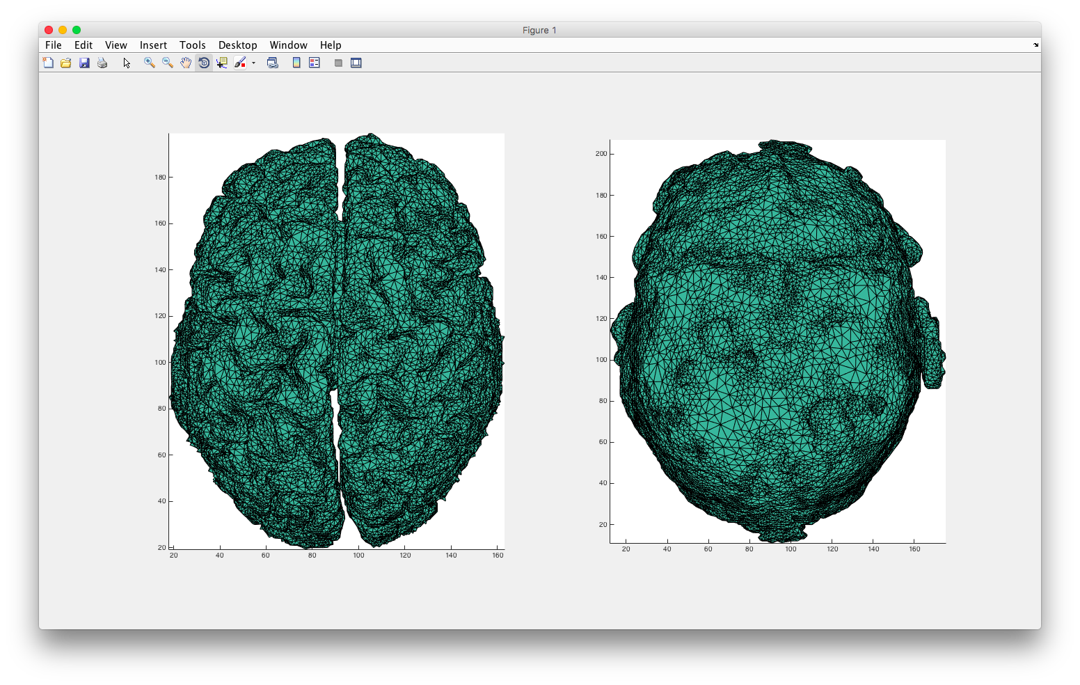
Brain Mesh Pipeline!
This serves as a tutorial for how to create segmented brain meshes out of MRI scans. It requires two open-source softwares, and one matlab library. It also uses the standard Colin27 set of MRI scans (which you can get for free). This was done on a Macbook Air, but should be pretty straightforward to run on windows (not sure about linux).
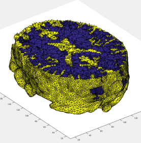
I did this because I am super curious about the brain lately. I'd like to participate in a study if they allow me to keep my MRI scans (so if you or someone you know needs participants, let me know!). MRI scans are pretty pricey =/
Necessary Tools
My workflow includes a suite of open source software that is used to view 3d files, segment MRI scans, and generate mesh files.Click for details
MRIcroGL
MRIcroGL is the OpenGL version of MRIcro. OpenGL (Open Graphics Library) is an API (application programming interface) for rendering vector graphics that interacts with a GPU (graphics processing unit). This interaction allows for hardware-accelerated rendering. The great part is that it is Open Source, meaning free and contributed to by you! I used MRIcroGL as a visualization tool to explore the image before segmenting it. Download here.
ITK-SNAP
ITK-SNAP is an open source software to segment structures inside 3d medical images. The cool part is that is have a semi-automatic segmentation method. It has extensive documentation online, including a short 90-minute course. Download here.
Iso2mesh
Iso2mesh is a meshing tool for matlab written by Professor Fang. It will allow us to create 3D tetrahedral finite element meshes from the segmentations we create using ITK-SNAP. Download here.
mmclab
Mech-based Monte Carlo simulation support for matlab written by Professor Qianqian Fang. Download here.
Data Formats
There are 2D and 3D formats I use. As well as standard MRI images you can use.Click for details
2D Format
The standard file format in medical applications is the DICOM format (Digital Imaging and Communication in Medicine). The big plus for this is that is have metadata attached to it (similar to how .jpg images have embedded tags). This metadata header can house the name of patient, time of test, date test was taken, medical record number, equipment used, manufacturer of equipment, settings, etc. It is expandable, so you can define what to include in the metadata. However, typically, DICOM is used to represent 2D slices. Matlab has a dicomread() function to read this information. Lately, DICOM has been saving images not just in greyscale, but RGB as well.
3D Format
For 3D medical data, there are 2 popular methods.
- The first is the Analyze Format. This format uses two parts. The first is a binary file (.img) and the second is a header file (.hdr). The binary file contains volumetric data. Each pixel is saved as a short integer and represented by two bytes in one file. The header file, similar to the information in a DICOM file, contains information about the data, including pixel spacing, date, time, etc.
- The second 3D file type is a NIfTI file (Neuroimaging Informatics Technology Initiative). It is adapted from the analyze format. It combines uses the “empty space in the analyze header to add several features.” The great part is that it is more convenient since it doesn’t require file pairs (.img+.hdr) and so you are less likely to accidentally separate your data.
Colin27
Colin27 is an open source atlas of MRI images. Actually, I believe its compiled from one person, and not from many people, but it is the go to sample of MRI images to test different software with. You can get the scans here. A more detailed description is found here.
MRIcroGL
This is used as a tool to visualize our data before segmenting it.Click for progress pictures ...
The first step in analyzing the Colin dataset provided is to open it in MRIcroGL. The folder provided contained four .hdr/.img file pairs. I the colin27.hdr files to get a better sense of what I wanted to segment.
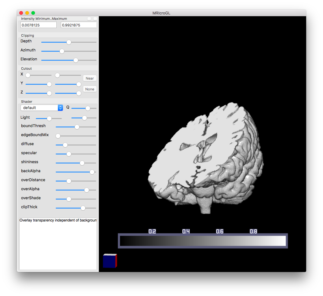
You can use a cutout section on the right menu to create a box to remove a certain part of the data set. You use the XYZ sliders to control the dimensions of the box. You can also add an overlay, which allows you to generate a 3D overlay of two 3D parts. This is great post segmenting a dataset, since it lets you see how the two physical spaces interact.
The Shader menu is a function that helps combine pixels along a vector to generate intensity. Eventually, intensity is shown as a 2D image, and this Shader menu allows you to pick different functions to process the voxels along a line of sight to determine how to represent the dataset in 2D. For example, the “mip” shader finds the max value along a vector and uses that as the intensity value. This is recalculated as you turn the 3D model around. You can render faster by lowering the quality using the slider next to “Q”.
However, out of all of this, I find the clip menu to be the most useful. Clipping allows you to visualize different planes. The depth slider pans linearly across the model from a specified point of view. The azimuth and elevation sliders change that point of view, allowing you to “clip” into the model from different angles.
Using this clip, I found two regions of interest that I want to segment. MRIcroGL helped me experiment with the dataset so I have a more targeted approach when segmenting. You can vaguely see these areas in the image above, but ITK-SNAP has some image processing tools to help me segment them.
ITK-SNAP
ITK-SNAP is a great tool to segment MRI images.Click for progress pictures ...
Now that I know my region of interest, I used ITK-snap to segment these volumes. As soon as I loaded the colin27_brainmask.img, I was sure to screenshot the data associated with what I loaded.
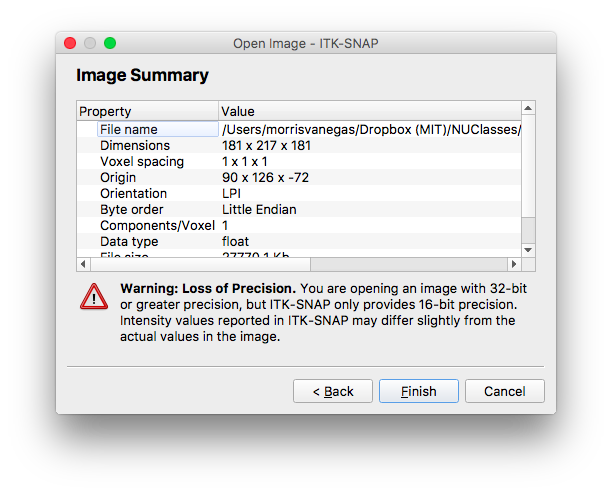
With the image open, you can use a pen brush to manually segment the volumes layer by layer, but this is 2017, and we have other important things to do. Instead, I used a snake approach, which is ITK-SNAPs semi-automated segmentation method. To start, click the snake icon on the top left. I then clicked “segment 3d,” which guides me in how to segment this model.
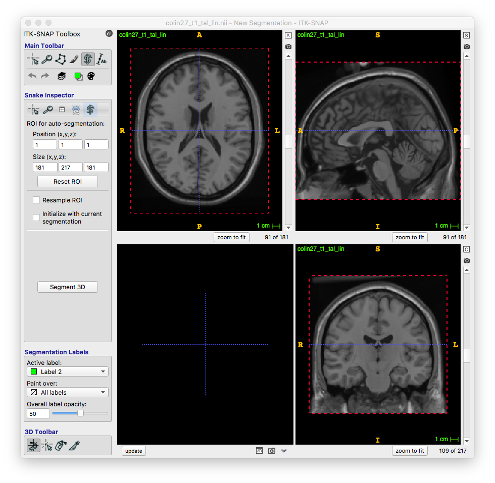
Pre-segmentation
Each image can now be viewed as a threshold image with a blue background. This helps in identifying what exactly you want to segment. There are different presegmentation modes in the right drop-down menu, including classification and clustering, but I prefer threshold for my region of interest (although I used clustering in my second segment of the rest of the breast). By clicking more, I open a window that allows me to tailor my threshold limits to exactly where I want to segment. This allowed me to isolate the region I want to work on.
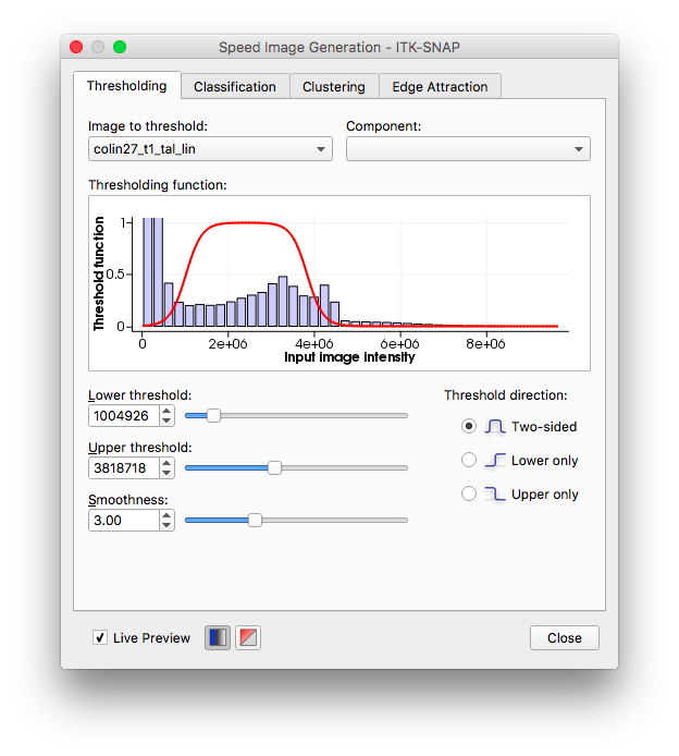
I picked a two-sided threshold, and adjusted the smoothness, which adjusts the shape of the transition function, to ensure I was able to see the range of input intensities I wanted. With that complete, I moved onto Initialization.
Initialization
This step allowed me to start identifying the region I wanted to segment. In any of the three views, I was able to click on a portion of the dataset to set my cursor. I then clicked “add bubble at cursor,” which, you guessed it, added a bubble at the cursor location. It created a sphere at the volumetric point. I repeated this step, ensuring I added bubbles in my region of interest in all levels. When I pressed “next,” ITK-snap combined these spheres together.
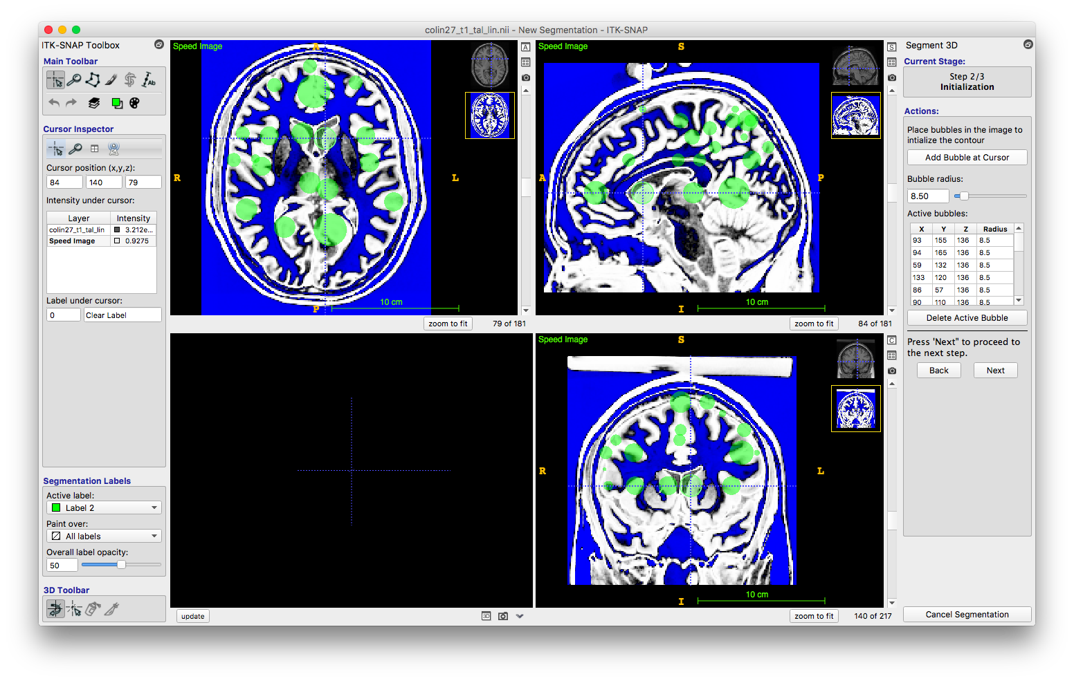
Evolution
This final step implements the snake approach to segment a region. The set parameters button lets me pick parameters to decide when regions should grow or contract, as well as whether we want to take a mathematical or “intuitive” approach. I used the intuitive approach, which uses the blue threshold to decide where the segmented volume should flow into.
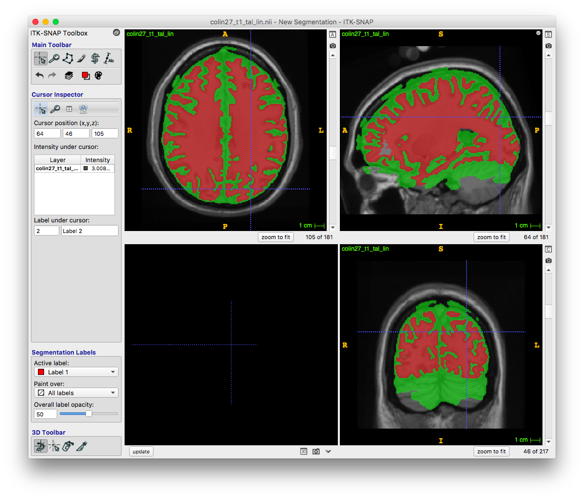
I pressed play, and the region grew like flowing water. I started and stopped it a couple times to look at different layers until the flowing water covered my region of interest. Clicked finished, and voila!
I then had to segment the rest of the area. I repeated the steps after picking a different layer. The only difference was that rather than using threshold for presegmentation, I used clustering because I gave me a better separation. The final segmentation of both regions is below.
Exporting
I exported the file as an analyze file, and it automatically compressed it for me. The compressed file was only 68 kb while the uncompressed was 22.3 Mb. To export, click segmentation -> Save Segmentation Image, and choose the Analyze file format.
Iso2Mesh
Iso2Mesh allows us to take the .img file from ITK-SNAP and create a mesh (3d geometry made of nodes and triangles).Click for progress pictures ...
Now I have a .img file, and I want to read it in.
fid=fopen(Untitled.img','r')
First, I use fopen to open the .img file we created for read access. The 'r' parameter means we want to make the file readable.
data=fread(fid,inf,'short');
Here, I read binary data. The second parameter inf means I read to the end of the file. With 'short' I’m telling matlab that I have 16 bit (2 byte) integers in the binary file.
data=reshape(data, [181 217 181]);
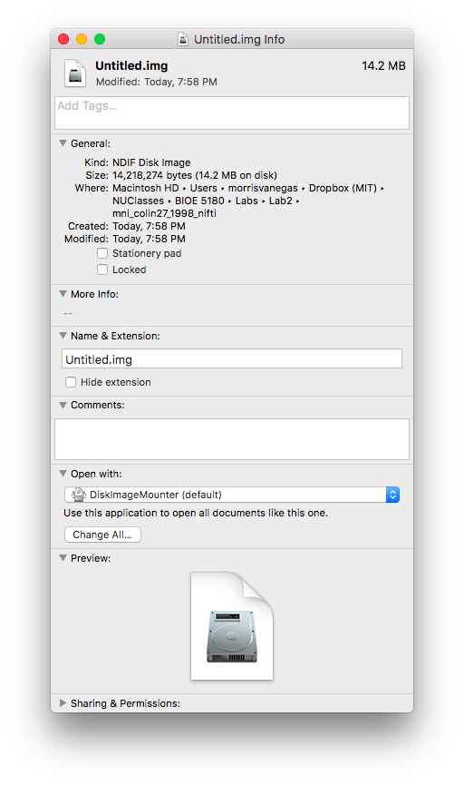
The reshape command returns a matrix. This is used to turn the read stream from fread into a matrix that is of a specified size. Here, I used the size from ITK-SNAP to determine what size the matrix should be. A cool way to check is to see that we have 181x217x181=7109137 voxels. However, each voxel is represented by a short integer (2 bytes), so we should have 7109137*2=14218274 bytes of data. Looking at the properties of the file, we see that it is 14.2 MB in size, the exact number of bytes. That means the .img file was truly binary, just raw data in a file. dope.
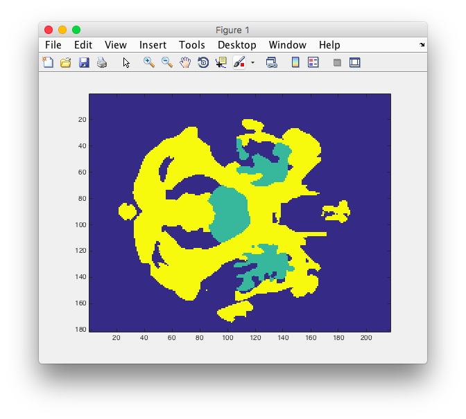
imagesc(data(:,:,40))
Just for good measure, I plotted at least one layer using imagesc. I was able to see the blue background, as well as my region of interest.
Great, now I am ready to make a mesh.
which s2m
I used this command to ensure Matlab knew where my iso2mesh .m files were located.
[node,elem]=v2m(uint8(data),[],15,100,'cgalmesh');
This command converts a 3d array to a mesh. The inputs are defined as v2m(img, ix,iy,iz,opt,maxvol,dofix,method,isovalues) The ones I used are described below.
- 1. Img: Name was given in uint8(data) format, and describes the output segmented data from ITK-SNAP
- 2. Ix,iy,iz: I gave an empty array [] to use the entirely of the data
- 3. Opt: 15 referred to the max triangular patch. This describes how big the triangles in the mesh can be. If you make this limit smaller, then smaller triangles are used, hence you get a denser mesh.
- 4. Maxvol: 100 described the max volume of each tetrahedron, which is made up of 4 triangles with a max size of 15.
- 5. Method: Cgalmesh referred to the method. According to the documentation of vol2mesh, cgalmesh is the most robust.
- RNG seed=1648335518
- Mesh sizes are (label=size) (1=100)
- node number: 91005
- triangles: 354600
- tetrahedra: 490024
- regions: 2
- surface and volume meshes complete
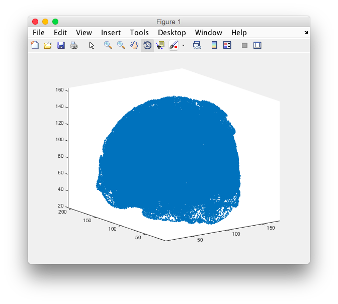
The v2m function generates two values: node and element. The node is a 4 column matrix that defines the x y and z coordinate of every vertex on the mesh., ie. just points in space. If you don’t believe me, type
plotmesh(node,'.')
to get a pretty point cloud.
The element output is a 5 column matrix that defines the connections between the nodes, ie. a solid tetrahedron. 4 nodes make a tetrahedron. The first 4 columns in elem show which indices are connected, and the last column is a number describing which label (segmentation) the element belongs to. Don’t believe me? Tough luck!
Just kidding. Type
unique(elem(:,end))
And you should see the number of segmented volumes you created in ITK-SNAP.
Finally, I used plotmesh() to generate some cool 3D mesh of my region of interest!
plotmesh(node,elem)
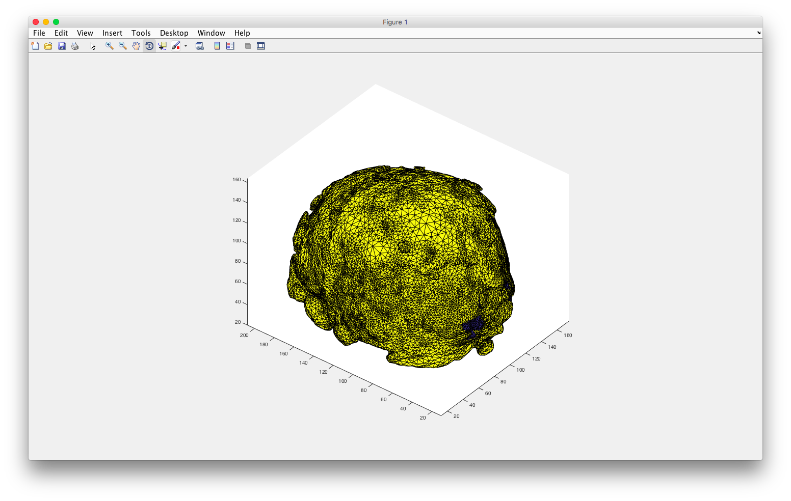
plotmesh(node,elem,'z< 90')
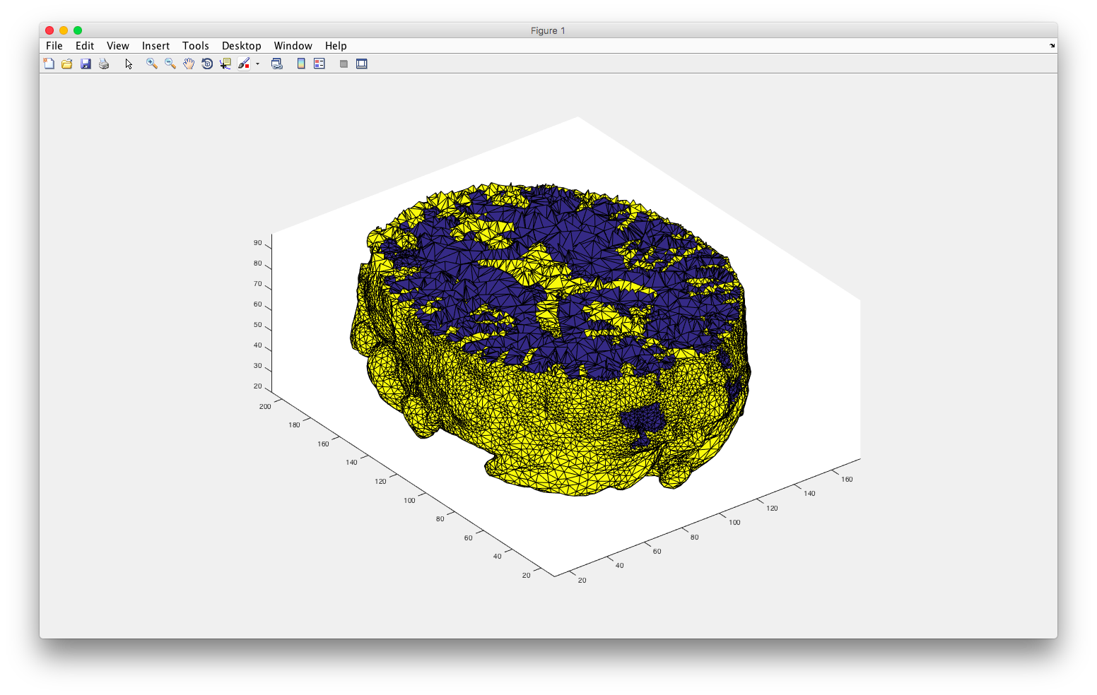
Or, using plotmesh(node,elem(elem(:,end)==1,:)) I can see the two regions individually.
